


Cameras
Digital Camera Interfaces
This is Section 10.1 of the Imaging Resource Guide.
As imaging technology advances, the types of cameras and their interfaces continually evolve to meet the needs of a host of applications. For machine vision applications in the semiconductor, electronics, biotechnology, assembly, and manufacturing industries where inspection and analysis are key, using the best camera system for the task at hand is crucial to achieving the best image quality. Understanding cameras parameters such as digital interfaces, power, and software provides a great opportunity to move from imaging novice to imaging expert.
Digital cameras are available with a variety of interface options that are often dependent on an application’s requirements. Some formats, such as the USB varieties, can greatly simplify the setup process by supplying video output and power via a single interface. Other formats may require an additional power supply but provide advantages such as higher data transfer rates, which affects the camera’s framerate, or support for a greater number of simultaneous devices. Table 1 compares the different digital camera interfaces.
| Digital Interface Comparison | ||||||
|---|---|---|---|---|---|---|
| DIGITAL SIGNAL OPTIONS NOTE: images not drawn to scale |
  |
 |
|
|
 |
 |
| USB 3.1 | GigE (PoE) | 5 GigE (PoE) | 10 GigE (PoE) | CoaXPress | Camera Link® | |
| Data Transfer Rate: | 5Gb/s | 1000 Mb/s | 5Gb/s | 10Gb/s | up to 12.5Gb/s | up to 6.8Gb/s |
| Max Cable Length: | 3m (recommended) | 100m | 100m | 100m | >100m at 3.125Gb/s | 10m |
| # Devices: | up to 127 | Unlimited | Unlimited | Unlimited | Unlimited | 1 |
| Connector: | USB 3.1 Micro B/USB-C | RJ45 / Cat5e or 6 | RJ45 / Cat5e or 6 | Cat7 or Optical Cabling | RG59 / RG6 / RG11 | 26pin |
| Capture Board: | Optional | Not Required | Not Required | Not Required | Optional | Required |
Table 1: Comparison of popular digital camera interfaces.
USB (Universal Serial Bus)
USB 3.1 Gen 1, formerly known as USB 3.0, is a popular interface due to its ubiquity among computers. It is high speed and convenient; maximum attainable speed depends upon the number of USB peripheral components, as the transfer rate of the bus is fixed at 5 Gb/s. In USB3 Vision, camera control registers are based on the EMVA GenICam standard. The USB3 Vision standard does not match that of the computer standard of backwards compatibility, but some USB 3.1 Gen 1 cameras are backward compatible making them run at the slower speed of USB 2.0 (480Mb/s). The most common USB 3.1 connector used in the machine vision camera industry is the USB 3.1 Micro B connector. Gradually being introduced to the market is USB-C (USB Type C), the connection type designed for the future. It features single and dual band top speeds of 10 and 20 Gb/s respectively. Additionally, this connector has a smaller footprint and is reversable. While cables and cameras that currently use USB-C are still limited to USB 3.1 Gen 1 data transmission speeds, this newer connector will be required as the industry adopts USB 3.1 Gen 2 as an alternative high-speed interface.
GigE (Gigabit Ethernet)
GigE is based on the gigabit ethernet internet protocol and uses standard Cat 5e and Cat 6 cables for a high-speed camera interface. Standard ethernet hardware such as switches, hubs, and repeaters can be used for multiple cameras, although overall bandwidth must be considered whenever non peer-to-peer (direct camera to card) connections are used. In GigE Vision, camera control registers are based on the EMVA GenICam standard. Optional on some cameras, Link Aggregation (LAG) uses multiple ethernet ports in parallel to increase data transfer rates. Also supported by some cameras, the network Precision Time Protocol (PTP) can be used to synchronize the clocks of multiple cameras connected on the same network, allowing for a fixed delay relationship between their associated exposures. 5 GigE and 10 GigE are newer versions of the GigE interface that feature data transfer rates of 5 Gb/s and 10 Gb/s, respectively.
CoaXPress
CoaXPress is a plug-and-play high-speed digital interface for use in high-resolution machine vision applications that require a fast frame rate. It uses a coaxial cable and is scalable for multiple cables; each cable is capable of up to 12.5 Gb/s, and each cable can provide up to 13W of power at a nominal 24V. Because of this scalability, there is no set maximum for a cable length with CoaXPress; the higher the bandwidth, the smaller the maximum cable length.
Camera Link®
Camera Link® is a high-speed serial interface standard developed explicitly for machine vision applications. A Camera Link® capture card is required for use, and power must be supplied separately to the camera. Special cabling is required because, in addition to low voltage differential pair (LVDP) signal lines, separate asynchronous serial communication channels are provided to retain full bandwidth for data transmission. The single-cable base configuration allows 2.04Gb/s transfer dedicated for video. Dual outputs (full configuration) allow for separate camera parameter send/receive lines to free up more data transfer space (6.8Gb/s) in extreme high-speed applications.
Capture Boards
Image processing typically involves the use of computers, which means a digital interface is necessary when using analog cameras. Capture boards allow users to output analog camera signals into a computer for analysis; for analog signals (NTSC, YC, PAL, CCIR), the capture board contains an analog-to-digital converter (ADC) to digitize the signal for further image processing. Users can then capture images and save them for future manipulation and printing. Basic capturing software is included with capture boards, allowing users to save, open, and view images.
The term capture board also refers to cards that are necessary to acquire and interpret the data from digital camera interfaces but are not based on standard computer connectors.
Laptops and Cameras
Although many digital camera interfaces are accessible to laptop computers, it is highly recommended to avoid standard laptops for high-performance and/or high-speed imaging applications. Often, the data buses on the laptop will not support full transfer speeds and the resources are not available to take full advantage of high-performance cameras and software. In particular, the ethernet network speed interface cards standard in most laptops perform at a much lower level than the PCIe cards available for desktop computers.
Powering the Camera
This is Section 10.2 of the Imaging Resource Guide.
Many camera interfaces allow for power to be supplied to the camera remotely over the signal cable (such as USB or PoE). Power over Ethernet (PoE) is a feature available in some but not all GigE cameras. When this is not the case, power is commonly supplied either through a Hirose connector (which also allows for trigger wiring and I/O), or a standard AC/DC adapter type connection. Even in cases where the camera can be powered by card or port, using the optional power connection may be advantageous. Below are three different ways to connect and power a GigE camera:
General-Purpose Input/Output (GPIO) Power Cable Connection
Connect the camera to a computer using a GigE cable. Next, plug in the GPIO power cable, also commonly referred to as a Hirose connector cable, to an electrical outlet and connect it to the camera’s power port. Different cameras will require GPIO cables with different numbers of pins, such as 6 or 12. For non-PoE cameras, a power cable may be the only method to power the camera.
Power over Ethernet (PoE) Injector
PoE injectors can deliver power to a camera over a GigE cable. This can be important when space restrictions do not allow for the camera to have its own power supply, as in factory floor installations or outdoor applications. In this case, the injector is added somewhere along the cable line with standard cables running to the camera and computer. However, not all GigE cameras are PoE compatible. Plug in the power cable of the PoE injector and connect its “IN” port to a computer using a GigE cable. Next, use another GigE cable to connect the “OUT” port of the injector to your camera.
Power over Ethernet Network Interface Card (PoE NIC)
PoE NICs provide power to a camera through a computer using a copper interface while allowing the camera to connect to a secure fiber network. PoE NICs also reduce the amount of outlets and cable required. Plug in the PoE card into an open slot on a computer motherboard and connect the internal power connection. Then, use a GigE cable to connect one of the card’s PoE ports and the camera.
Camera Software
This is Section 10.3 of the Imaging Resource Guide.
In general, there are two choices when it comes to imaging software: camera-specific Software Development Kits (SDKs) or third-party software. SDKs include application programming interfaces with code libraries for development of user defined programs, as well as simple image viewing and acquisition programs that do not require any coding and offer simple functionality. With third-party software, camera standards (GenICam, DCAM, USB3 Vision, GigE Vision) are important to ensure functionality. Third party-soft-ware includes software such as NI LabVIEW™, MATLAB®, and OpenCV. Often, third-party software is able to run multiple cameras and support multiple interfaces, but it is ultimately up to the user to ensure functionality.
Sensors
This is Section 10.4 of the Imaging Resource Guide.
Sensor Size
The size of a camera sensor’s active area is important in determining the system’s field of view (FOV) and primary magnification $ \small { \left( m \right)} $. Given a fixed magnification that is determined by the imaging lens, larger sensors yield greater FOVs. As shown in Figure 1 and in Table 2, there are several standard area-scan sensor sizes. The nomenclature of these standards dates back to the Vidicon vacuum tubes used for television broadcast imagers, so it is important to note that the actual dimensions of the sensors differ. However, most of these standards maintain a 4:3 (horizontal:vertical) dimensional aspect ratio.
One issue that often arises in imaging applications is the ability of an imaging lens to support certain sensor sizes. If the sensor is too large for the lens design, the resulting image may appear to fade away and degrade towards the edges because of vignetting (extinction of rays that pass through the outer edges of the imaging lens). This is sometimes referred to as the tunnel effect since the edges of the field become dark. Smaller sensor sizes do not yield this vignetting issue.
CCD vs. CMOS Sensors
CCD (charge coupled device) and CMOS (complementary metal oxide semiconductor) are different sensor technologies for converting light into electronic signals. In a CCD, each pixel’s charge is converted to voltage, buffered, and transferred through a single node as an analog signal. In a CMOS sensor, the charge-to-voltage conversion is done at the pixel level. Historically, this conversion yielded a less uniform output.
New advances in CMOS technology over the last several years have helped greatly reduce the non-uniformity in low light environments, and in many applications high-end CMOS sensors can outperform the comparable CCD. Additionally, CMOS has lower power consumption than CCD, which makes them useful for any space-constrained application. Lower-end CMOS sensors with pixels smaller than approximately 3 microns are still outperformed by CCD in terms of image quality. Performance differences are highlighted in Table 3.

Figure 1: Sensor size dimensions for standard camera sensors.
| Camera Resolution by Pixel Size | |||||||||
|---|---|---|---|---|---|---|---|---|---|
| Pixel Size [µm] | 9.9 | 7.4 | 5.86 | 5.5 | 4.54 | 3.69 | 3.45 | 2.2 | 1.67 |
| Resolution $ \left[ \tfrac{\text{lp}}{\text{mm}} \right] $ | 50.5 | 67.6 | 85.3 | 90.9 | 110.1 | 135.5 | 144.9 | 227.3 | 299.4 |
| Typical ½" Sensor [MP] | 0.31 | 0.56 | 0.89 | 1.02 | 1.49 | 2.26 | 2.58 | 6.35 | 11.02 |
Table 2: Camera resolution by pixel size.
| CCD vs. CMOS Sensors | |||||
|---|---|---|---|---|---|
| CCD | CMOS | CCD | CMOS | ||
| Pixel Signal: | Electron Packet | Voltage | Uniform: | High | Moderate |
| Chip Signal: | Analog | Digital | Resolution: | Low-High | Low-High |
| Fill Factor: | High | Moderate | Speed: | Moderate-High | High |
| Responsivity: | Moderate | Moderate-High | Power Consumption: | Moderate-High | Low |
| Noise Level: | Low | Low to High | Complexity: | Low | Moderate |
| Dynamic Range: | High | Moderate to High | Cost: | Moderate | Low |
Table 3: CCD vs. CMOS Sensors.
Spectral Properties
This is Section 10.5 of the Imaging Resource Guide.
Depending on an application’s requirements, a camera’s ability to reproduce color may or may not be beneficial. A comparison of monochrome, single chip color, and three chip color cameras is shown in Table 4 and more detail is provided in the following section.
| Monochrome vs. Color | ||
|---|---|---|
| Monochrome | Color (Single Chip) | 3 Chip Color Cameras |
| Single Sensor Outputs Grayscale Images | Uses RGB Bayer Color Filter (Typical) | Utilizes a Prism to Split White Light into 3 Different Sensors |
| 10% Higher Resolution than Comparable Single-Chip Color Cameras | Lower Resolution (More Pixels Required To Recognize Color) | More Costly |
| Better Signal-To-Noise Ratio; Greater Contrast | Better Color Resolution | |
| Increased Low-light Sensitivity | Smaller Selection of Lenses | |
| Mag Require Specially Designed Lenses | ||
Table 4: Comparison of monochrome, (single-chip) color, and 3 chip color cameras.
Monochrome Cameras
CCD and CMOS sensors, being silicon devices, are sensitive to wavelengths from approximately 350 - 1050nm, although the usable range is usually given from 400 - 1000nm. This sensitivity is indicated by the sensor’s spectral response curve (Figure 2). However, most high-quality color, and some monochrome, cameras provide an infrared (IR) cut-of filer for imaging specifically in the visible spectrum.

Figure 2: Normalized spectral response of a typical monochrome CCD.
Color Cameras
The solid state sensor is based on the photoelectric effect and, as a result, cannot distinguish between colors without additional considerations. There are two types of color CCD cameras: single chip and three-chip. Single chip color CCD cameras offer a common, low-cost imaging solution and use a mosaic (e.g. Bayer) optical filer to make different pixels sensitive to only certain wavelengths of light. A color image is then reconstructed in software using a “de-bayering” algorithm which interpolates true color information from the RGB signals. Since more pixels are required to recognize color, single chip color cameras inherently have lower resolution than their monochrome counterparts. Three-chip color CCD (3CCD) cameras are designed to solve this resolution problem by using a prism to direct each section of the incident spectrum to a different chip. Although 3CCD cameras typically provide extremely high resolutions and more accurate color reproduction, they have lower light sensitivities and can be costly.
Frame Rate and Shutter Speeds
The frame rate refers to the number of full frames composed in a second. In high-speed applications, it is beneficial to choose a faster frame rate to acquire more images of the object as it moves through the FOV. The shutter speed corresponds to the inverse of the exposure time of the sensor. The exposure time controls the amount of incident light collected by the sensor. Camera blooming (caused by over- exposure) can be controlled by decreasing illumination, or by increasing the shutter speed (decreasing exposure time).
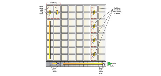
The maximum frame rate for a system depends on the sensor readout speed, the data transfer rate of the interface, and the number of pixels (amount of data transferred per frame). Often, a camera may be run at a higher frame rate by reducing the resolution by binning pixels together or restricting the area of interest. For digital cameras, exposures can be made from tens of microseconds to minutes, although the longest exposures are generally only practical with CCD cameras, which have lower dark currents and noise compared to CMOS.
Electronic Shutter: Global vs. Rolling
A global shutter is analogous to a mechanical shutter, in that all pixels are exposed and sampled simultaneously, with the readout then occurring sequentially; the photon acquisition starts and stops at the same time for all pixels. On the other hand, a rolling shutter exposes, samples, and reads out sequentially; it implies that each line of the image is sampled at a slightly different time. Intuitively, images of moving objects are distorted by a rolling shutter; this effect can be minimized with a triggered strobe placed at the point in time where the integration period of the lines overlaps. Note that this is not an issue at low speeds. Implementing global shutter for CMOS requires more complicated sensor architecture than the standard rolling shutter model, and thus they are not available on all CMOS sensors. A comparison of global and rolling shutters is shown in Figure 3.


Figure 3: Comparison of motion blur. Stationary PCB (A) and images of moving PCB with continuous global shutter (B) and rolling shutter (C).
In contrast to global and rolling shutters, an asynchronous shutter refers to the triggered exposure of the pixels. That is, the camera is ready to acquire an image, but it does not enable the pixels until after receiving an external triggering signal. This is opposed to a normal constant frame rate, which can be thought of as internal triggering of the shutter.
For more information on the basics of digital camera and sensor settings including gain, gamma, area of interest (AOI), and more, read Imaging Electronics 101: Basics of Digital Camera Settings for Improved Imaging Results.
Area Scan vs. Line Scan Camera
This is Section 10.6 of the Imaging Resource Guide.
Depending on an application’s requirements, a system implementer must choose between an area scan or line scan camera. In area scan cameras, an imaging lens focuses the object to be imaged onto the sensor array, and the image is sampled by the pixels all at once for reconstruction (Figure 4a). This is convenient if the image is not moving quickly or if the object is not extremely large. With line scan cameras, the pixels are arranged in a linear fashion, and as the object moves past the camera, the image is taken line by line and reconstructed with software (Figure 4b).

Figure 4: Illustration of an area scan camera (left) and a line scan camera (right).
Linear arrays are capable of much higher resolutions than area scan devices, with 4,000 pixels being the highest typical horizontal resolution of area scan sensors, while upwards of 16,000 pixels in a linear device is not uncommon. However, with line scan cameras, the object must be precisely moved relative to the camera to construct the image, making integration much more difficult. A brief overview of area scan and line scan cameras is provided in Table 5.
| Digital Camera Formats | ||
|---|---|---|
| Area Scan | Line Scan | |
| 4:3 (H:V) Ratio (Typical) | Sensor is Linear | |
| High Speed Applications Up to a Few Hundred FPS | High Speed Applications- Line rates Up to 100khz | |
| Object is Stationary or Slowly Moving | Constructs Image One Line at a Time | |
| Wider Range of Applications | Object Passes in Motion Under Sensor | |
| Easier to Set-up | Ideal for Capturing Wide Objects | |
| Lower Cost than Line Scan | Special Alignment & Timing Required | |
| Complex Integration / Simple, but Intense, Illumination | ||
Table 5: Comparison of digital camera formats: area scan and line scan.
| Standard Camera/Lens Mounting Configurations | ||||
|---|---|---|---|---|
| C-Mount | CS-Mount | TFL-Mount | F-Mount | Other Common Mounts |
| Threaded Mount | Threaded Mount | Threaded Mount | Nikon-Style Bayonet Mount (Not Threaded) | M12 x 0.5 (S-Mount) |
| 1" Diameter with 32 TPI (Threads Per Inch) | 1" Diameter with 32 TPI (Threads Per Inch) | M35 x 0.5 mm | Used On Large Sensor Cameras | M42 x 1.0 |
| 17.5mm Back Flange Distance | 12.5mm Back Flange Distance | 17.5 mm Back Flange Distance | 46.5mm Back Flange Distance | M72 x 1.0 |
| Most Common Interface | Compatible with C-Mount Lenses | Ideal for 4⁄3 to APS-C sensor formats | Ideal for Medium Format Line Scan and Full Frame (35mm) Format Applications | |
| Some Short FL Lenses Not Compatible | Common on Short FL / Varifocal Lenses | |||


or view regional numbers
QUOTE TOOL
enter stock numbers to begin
Copyright 2024, Edmund Optics Singapore Pte. Ltd, 18 Woodlands Loop #04-00, Singapore 738100
California Consumer Privacy Acts (CCPA): Do Not Sell or Share My Personal Information
California Transparency in Supply Chains Act
This content may include material that has been generated or modified using artificial intelligence (AI).
The FUTURE Depends On Optics®